生成模型基础 | 2 Transformers
就像卷积神经网络 (比如 UNet) 一样, Transformer 指的是一种具体的神经网络架构, 可以用它做各种各样的学习任务 (监督、非监督). Transformer 是序列到序列 (sequence to sequence) 的映射, 最初由 NLP 的研究人员提出.
Different modules in Transformers cope with different challenges in NLP:
- Long term dependency:
我的书柜太宽了,而且非常重,我没有办法把它搬出书房
- Self attention
- Sophisticated meaning:
我原以为这部电影挺无聊的,没想到还不错
- FFN
- Word order matters a lot: 屡战屡败?屡败屡战!
- Positional encoding
5 Transformers
5.1 Self attention
Self attention 做的是整合上下文信息.
假设每个单词有嵌入表示 \(x_i\in\R^D\) (行向量). Self attention 输入的是一个序列 \((x_1,\dots,x_L)\), 输出的也是一个序列 \((z_1,\dots,z_L)\). 输出的序列中每个向量 \(z_i\) 不光包含了当前单词 \(x_i\) 的语义, 还整合了上下文的信息 (所谓 context):
- The word “Apple” here is a fruit or a company?
- “Alice” is happy or sad?
- The word “new” is an adjective or a part of name entity?
我们希望这个 attention 操作是:
- Selective: 有选择地整合上下文信息, 即应当选择上下文中哪些词重要, 哪些词不重要.
- Word-dependent: 选择的过程应当与当前词是什么有关.
5.2 A differentiable approach
Self attention 的具体操作可以视作一种 “可微检索”. 在此之前我们先看看不可微的检索——hash 表.
一个 hash 表包含若干键值对 (key-value pairs) \(\{(k_i,v_i)\}_{i=1}^N\).
- 这里 key, value 都是行向量: \(k_i,v_i\in\R^D\).
查表的过程是, 给定一个 query \(q\in\R^D\), 我们遍历一遍 keys \(\{k_i\}_i\), 如果某个 \(k_i=q\), 则返回对应的 value \(v_i\). 如果没有匹配的 key, 则查表失败, 什么也不返回.
Hash 表是比较 “hard” 的, 输出值关于 \(q\) 不连续, 这样既不稳定, 也不方便放进神经网络里用梯度下降优化. 对此, 我们用一种比较 “soft” 的查表方法:
(Scaled dot product) 计算每个 query \(q_i\) 与每个 key \(k_j\) 的内积 \[ s_{ij} := \frac1{\sqrt{D}}(q_i k_j\T), \] 这衡量了 query \(i\) 与 key \(j\) 的相关程度, 可以视作第 \(j\) 个单词对第 \(i\) 个单词的 “贡献”.
- Query, key 和 value 是词嵌入 \(x\) 分别通过三个线性层 \(W_q,W_k,W_v\) 得到的.
分母上的 \(\sqrt{D}\) 是归一化系数, 作用是防止模型在训练初期收敛到局部极值. 假设 \(q_i,k_j\) 的初始值服从 \(D\) 维标准正态分布 \(\mathcal{N}(0,I_D)\) 且相互独立, 则 \[ \Align{ \operatorname{var}(q_ik_j\T) = \operatorname{E}[(q_ik_j\T)^2] &= \operatorname{E}\!\bqty{ \biggl( \sum_{l=1}^{D} q_{ij}k_{jl} \biggr)^{\!\!2\,} } \\ &= \sum_{l=1}^{D} \operatorname{E}[(q_{ij}k_{jl})^2] \\ &= \sum_{l=1}^{D} \operatorname{E}(q_{ij}^2) \operatorname{E}(k_{jl}^2) \\ &= D. } \]
(Normalization) 将相关程度用 softmax 归一化, \[ a_{ij} = \frac{\exp(s_{ij})}{\sum_k \exp(s_{ik})}, \] 这仍旧是即第 \(j\) 个单词对第 \(i\) 个单词的贡献, 只不过归一化到了 \(a_{ij}\in(0,1)\), 并且可以理解为某种 “概率”: \[ \sum_j a_{ij} = 1. \]
Note “Softmax” vs “hardmax”.
Softmax 映射的非连续版本 (“hard” 版本) 是 one-hot 映射, 即 \[ a_{i} = (\underbrace{0,\dots,0,1}_k,0,\dots,0), \] 其中 \(k=\argmax_j s_{ij}\). 也就是只保留最大的 \(a_{ij}\) 为 \(1\), 将其余的都置为 \(0\). 若在 softmax 函数中引入 “温度” 参数 \(\tau\), \[ a_{ij} = \frac{\exp(s_{ij}/\tau)}{\sum_k \exp(s_{ij}/\tau)}, \] 则 one-hot 映射是当 \(\tau\to0\) 时的极限.
(Weighted sum) 将 value 按照 score 加权求和, 作为第 \(i\) 个单词的输出: \[ z_{i} := \sum_j a_{ij} v_j. \]
这也称作 scaled dot-product attention, 如下图
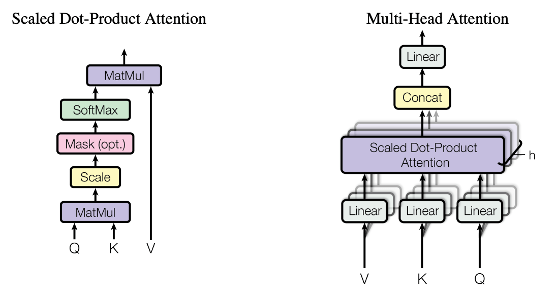
更紧凑的形式: 将所有单词的行向量叠起来得到矩阵 \(X\in\R^{L\times D}\), 分别经过三个线性层得到 query, key, value 矩阵: \[ Q=XW_q, \qquad K=XW_k, \qquad V=XW_v, \] 其中 \(Q,K,V\in\R^{L\times D}\). Self-attention 的矩阵形式为 \[ \operatorname{attention}(X) = \operatorname{softmax}\biggl( \frac{1}{\sqrt{D}} QK\T \biggr) V. \]
记号约定: 矩阵用大写字母表示, \[ \operatorname{attention}(X) = \underbracket{ \underbracket{\operatorname{softmax}\biggl( \overbracket{\frac{1}{\sqrt{D}} QK\T}^S \biggr)}_A V }_Z, \] 相应的行向量用小写字母.
5.3 The Transformer
Transformer 的架构如下图所示
![]()
每个 transformer block 包含以下几个模块:
多头注意力.
前馈网络 (feedforward network, FFN), 就是普通的全连接层, 它的作用是对整合好的上下文的信息进一步加工、提炼.
层归一化 (layer normalization, LN), 将矩阵 \(X\in\R^{L\times D}\) 的每行 \(x\in\R^D\) 按照各自的均值与方差归一化, 再整体缩放+平移: \[ \operatorname{LN}(x) := \frac{x-\operatorname{E}(x)} {\sqrt{\operatorname{D}(x) + \varepsilon}} \odot\beta + \gamma. \] 归一化可以控制输出值的大小, 让优化更稳定, 避免数值溢出. 仿射变换参数 \(\beta,\gamma\in\R^D\) 是可学习的.
残差连接 (residual connection), 引出一路数据流, 跳过 FFN/attention, 并与 FFN/attention 的输出叠加. 叠加后的结果送给层归一化.
多头注意力是 Transformer 中唯一跨 tokens 计算的模块, FFN、LN 都是 \(x_i\) 各自平行计算的.
Note 形形色色的归一化.
NLP 与 CV 中的训练数据一般是高维张量:
- (NLP) Batch size \(B\), 序列长度 \(L\), 嵌入维数 \(D\).
- Batch size \(B\), 像素数 \(H\times W\), 通道数 \(C\).
取出不同的维度计算方差和均值, 就可以得到不同的归一化方法:
Batch norm. (BN)
- 对空间维和 batch 维求 \((\mu,\sigma)\), 每个 channel/embedding 算出一组 \((\mu,\sigma)\): \[ \Align{ X:&\quad \mathtt{B\times C\times H\times W} &&& &\quad\mathtt{B\times L\times D} \\ &\quad \mathtt{ \mathrlap{\downarrow}\hphantom{B} \hphantom{{}\times{}} \mathrlap{ }\hphantom{B} \hphantom{{}\times{}} \mathrlap{\downarrow}\hphantom{B} \hphantom{{}\times{}} \mathrlap{\downarrow}\hphantom{B} } &&\textsf{or}\hspace{-1em}& &\quad\mathtt{ \mathrlap{\downarrow}\hphantom{B} \hphantom{{}\times{}} \mathrlap{\downarrow}\hphantom{B} \hphantom{{}\times{}} \mathrlap{ }\hphantom{B} } \\ \mu,\sigma:&\quad \mathtt{1\times C\times 1\times 1} &&& &\quad \mathtt{1\times 1\times D} } \] BN 是 CNN 的标配, 可以大幅加速收敛, 缺点是依赖于 batch size. 早期 RNN/CNN-NLP 也使用过 BN, 但对变长序列和小 batch 不稳定, 所以后来几乎被 LN/RMSNorm 替代.
Layer norm. (LN)
- 主要在 Transformer 中使用, 对 embedding 维度求 \((\mu,\sigma)\), \[ \Align{ X:&\quad \mathtt{B\times L\times D} \\ &\quad \mathtt{ \mathrlap{ }\hphantom{B} \hphantom{{}\times{}} \mathrlap{ }\hphantom{B} \hphantom{{}\times{}} \mathrlap{\downarrow}\hphantom{B} } \\ \mu,\sigma:&\quad \mathtt{B\times L\times 1} } \] LN 可以减少数值波动, 且独立于 batch size 和 sequence length, 适合 batch size / sequence length 不固定的场景.
Instance norm. (IN)
- 一般只在 CV 中使用, 对空间维求 \((\mu,\sigma)\), 每个样本的每个 channel 算出一组 \((\mu,\sigma)\): \[ \Align{ X:&\quad \mathtt{B\times C\times H\times W} \\ &\quad \mathtt{ \mathrlap{ }\hphantom{B} \hphantom{{}\times{}} \mathrlap{ }\hphantom{B} \hphantom{{}\times{}} \mathrlap{\downarrow}\hphantom{B} \hphantom{{}\times{}} \mathrlap{\downarrow}\hphantom{B} } \\ \mu,\sigma:&\quad \mathtt{B\times C\times 1\times 1} } \] IN 可以认为消除了图像的风格/亮度的差异, 它的一个重要应用是风格迁移 (style transfer).
5.4 *Time complexity
最后来讨论 Transformer 的计算效率.
输入长度为 \(L\) 的序列, 嵌入维度为 \(D\), 则输入矩阵 \(X\in\R^{L\times D}\). 三个线性层 \(W_k,W_q,W_v\in\R^{D\times D}\). FFN 的线性层 \(W_{\textsf{FFN}}\in\R^{D\times D}\).
- 矩阵乘法 \(Q=XW_q\), \(K=XW_k\), \(V=XW_v\) 的时间复杂度均为 \(O(LD^2)\)
将 \(m\times n\) 和 \(n\times k\) 的矩阵相乘需要进行 \(mnk\) 次乘法/加法操作. [3]. - Scaled dot product \(S=QK\T/\sqrt{D}\) 的时间复杂度为 \(O(L^2D)\).
- Softmax \(A=\operatorname{softmax}(S)\) 的时间复杂度为 \(O(L^2)\).
- 矩阵乘法 \(Z=AV\) 的时间复杂度为 \(O(L^2D)\).
- FFN 层中的矩阵乘法复杂度为 \(O(LD^2)\).
一般嵌入维数 \(D\) 固定, 而序列长度 \(L\) 变化, 可以很短也可以很长. 因此, 整个 Transformer 的计算复杂度是序列长度 \(L\) 的平方级别: \(O(L^2)\).
6 Positional encoding
Attention 模块没有考虑单词的位置信息. 假设将输入序列 \((x_1,\dots,x_L)\) 随机排列, 那么输出序列 \((z_1,\dots,z_L)\) 也会相应排列——而具体数值是完全一样的!
这就需要位置编码 (positional encoding) 模块出场了, 它可以在 attention 操作中引入位置信息.
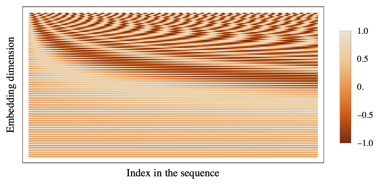
6.1 Absolute PEs
绝对位置编码 (absolute positonal encoding) 是最初的位置编码
绝对位置编码的缺点:
- 不可学习的位置编码在更长序列上泛化性差.
- 可学习的位置编码无法用于更长序列.
- 无法让模型学习到单词的相对位置 (比如 “X 在 Y 两个 token 之前”), 只能学到绝对位置 (比如 “X” 是第一个 token), 不易推广到变长序列.
正弦位置编码公式背后的动机是什么? 计算 \(p_i\) 和 \(p_j\) 的内积, \[ p_ip_j\T = \sum_{i=d}^D \cos((j-i)\theta_d) = f(j-i), \] 可以发现它只和相对位置 \((j-i)\) 有关, 原论文作者认为这能让模型学到相对的位置关系. 然而如果我们计算 query \(\tilde{q}_i\) 和 key \(\tilde{k}_j\) 的内积, \[ \Align{ \tilde{s}_{ij} = \frac{1}{\sqrt{D}}\tilde{q}_i \tilde{k}_j\T &= \frac{1}{\sqrt{D}} \biggl[ (x_i+p_i)W_q \cdot W_k\T(x_j+p_j)\T \biggr] \\ &= \frac{1}{\sqrt{D}} \biggl[ \underbrace{x_iW_qW_k\T x_j\T}_{\textsf{原本的内积 }q_ik_j\T} + \underbrace{x_iW_qW_k\T p_j\T + p_iW_qW_k\T x_j\T}_{\textsf{交叉项}} + p_i {\color[rgb]{.7,.7,.7}{W_q W_k\T}} p_j\T \biggr]. } \] 其中最后一项和 \(p_ip_j\T\) 很像, 但是中间多出了 \({\color[rgb]{.7,.7,.7}{W_q W_k\T}}\), 导致这一项不再是 \((i-j)\) 的函数. 此外, 两个交叉项刻画的是绝对位置而非相对位置. 总之, 这种绝对位置编码方式不能很好地刻画相对位置.
6.2 Relative PEs
为了让模型学到相对位置信息, 人们提出了一种新的方法
\[ \tilde{s}_{ij} = \frac{1}{\sqrt{D}} \underbrace{x_iW_qW_k\T x_j\T}_{\textsf{原本的内积 }q_ik_j\T} + \orange{b_{i,j}}, \] 其中偏置项 \(b_{i,j}=f(j-i)\) 是关于相对位置的函数, 一般是可学习的. 用矩阵形式写出来就是在 attention 矩阵 \(QK\T/\sqrt{D}\) 上叠加了一个 bias 矩阵: \[ \tilde{A} = \operatorname{softmax}\bigl(QK\T/\sqrt{D} + \orange{B}\bigr). \]
6.3 Rotary PEs
相对位置编码仍有改进空间. RoPE 的论文重新 formulate
了需要解决的问题
\[ \Align{ \varphi: (q_i,i) &\mapsto \tilde{q}_i, \\ (k_j,j) &\mapsto \tilde{k}_j. \\ } \]
即输入向量 \(q_i\) 或 \(k_j\) 和它们的位置 \(i\) 或 \(j\) 之后, 输出编码了位置信息的向量 \(\tilde{q}_i\) 或 \(\tilde{k}_j\). 虽然 \(\varphi\) 编码的都是绝对位置信息, 但我们希望它们的内积代表了相对位置信息: \[ [\varphi(q_i,i)][\varphi(k_j,j)]\T = f(q_i,k_j,\blue{j-i}). \]
该函数方程的一个解为 (常数 \(\theta\in\R\)) \[ \varphi(x,i) := xR_i \equiv x\begin{pmatrix} R_{i,1} \\ & R_{i,2} \\ && \ddots \\ &&& R_{i,D/2} \end{pmatrix}, \] 其中 \(2\) 阶方阵 \(R_{i,d}\) (\(d=0,1,\dots,D/2-1\)) 为逆时针旋转 \(i\theta_d=i\cdot{10000^{-2d/D}}\) 的矩阵: \[ R_{i,d} := \begin{pmatrix} \cos(i\theta_d) & \sin(i\theta_d) \\ -\sin(i\theta_d) & \cos(i\theta_d) \\ \end{pmatrix}. \] 从几何上看, 就是把 \(q_i\) 按照嵌入维度 \(D\) 分成两个一组 \(\{(q_{i,2d},q_{i,2d+1})\}_{d=1}^{D/2}\), 每组逆时针旋转 \(i\theta_d\) 弧度 (对 \(k_j\) 同理), 因此这种位置编码也叫做 RoPE (rotary position embedding).
此时计算 \(\tilde{q}_i\) 和 \(\tilde{k}_j\) 的内积得到 \[ \Align{ \tilde{q}_i\tilde{k}_j\T &= [\varphi(q_i,i)][\varphi(k_j,j)]\T \\ &= (q_iR_i)(k_jR_j)\T = q_i (R_iR_j\T) k_j\T = q_i \orange{R_{j-i}\T} k_j\T, } \] 其中 \(\orange{R_{j-i}\T}\) 恰好编码了相对位置信息.
RoPE 的矩阵形式为 \[ \tilde{A} = \operatorname{softmax} \bigl(\orange{\varphi}(Q)\orange{\varphi}(K)\T/\sqrt{D}\bigr), \] 其中旋转操作 \(\varphi(Q),\varphi(K)\) 可以通过复数乘法实现: 将 \(Q,K\) 转化为 \(\R^{L\times(D/2)}\) 的复矩阵, 乘以复矩阵 \(R^{(D/2)\times(D/2)}\), 再将结果转化回实矩阵.
Ashish Vaswani et al, Attention Is All You Need, 2017.↩︎
Ashish Vaswani et al, Attention Is All You Need, 2017.↩︎
将 \(m\times n\) 和 \(n\times k\) 的矩阵相乘需要进行 \(mnk\) 次乘法/加法操作.↩︎
Ashish Vaswani et al, Attention Is All You Need, 2017.↩︎
Colin Raffel et al, Exploring the Limits of Transfer Learning with a Unified Text-to-Text Transformer (2020).↩︎
Jianlin Su et al, RoFormer: Enhanced Transformer with Rotary Position Embedding (2021).↩︎