自然语言处理基础 | 2 语言模型
2 Language Modeling
词汇集为 \({\cal V}\), 所有可能的句子的集合为 \({\cal S}\), 则语言模型 (language model) 指的是 \({\cal S}\) 上的一个概率分布 \(p\), \[ \sum_{s\in{\cal S}} p(s)=1,\quad p(s)\geq0. \] 它给出了每句话的概率. 比如对于英文语言模型来说, "the dog barks" 或者 "the dog laughs" 的概率应该比较高, 而 "dog the laughs bark" 等不合语法/逻辑或不常用的句子的概率应该比较低.
Why language models?
Speech Recognition: \[ \textsf{words}^* = \argmax_{\textsf{words}} \bqty{ \textsf{Faithfulness}(\textsf{signal},\textsf{words}) + \orange{\textsf{Fluency}(\textsf{words})} }. \]
Optical Character Recognition (OCR)
Handwriting Recognition
Word Segmentation ("whatdoesthismean?")
Machine Translation
- Statistical Machine Translation
Language Generation
Question Answering/Dialogue/Chat
2.1 N-gram
将一个句子建模成一个随机变量序列 \((X_1,\dots,X_n)\), 则一个具体的句子 \((w_1,\dots,w_n)\) (\(w_i\in{\cal V}\)) 的概率为 \[ P(X_1=w_1,\dots,X_n=w_n). \] 一般令 \(w_n={\sf STOP}\) 为一个特殊的标识符. 有时也令 \(w_1={\sf START}\).
2.1.1 Markov assumptions
将上式按照 product formula 展开: \[ \Align{ &P(X_1=w_1,\dots,X_n=w_n) \\ &\hspace{1em}= P(X_1=w_1) \prod_{i=2}^n P(X_i=w_i\mid X_1=w_1,\dots,X_{i-1}=w_{i-1}). } \] 然而, 如此长的条件概率是难以计算的. 大多数时候我们并不需要如此长的 history 来预测新的词. 为此我们假设当前的词只与前一个词有关 (first-order Markov assumption). 于是, \[ \Align{ &P(X_1=w_1,\dots,X_n=w_n) \\ &\hspace{1em}= P(X_1=w_1) \prod_{i=2}^n P(X_i=w_i\mid X_1=w_1,\dots,X_{i-1}=w_{i-1}) \\ &\hspace{1em}= P(X_1=w_1) \prod_{i=2}^n \orange{P(X_i=w_i\mid X_{i-1}=w_{i-1})}. } \] 如此得到的语言模型称为 bigram, 因为它每次只考虑两个词的依赖关系.
最极端地, 可以假设当前词与历史无关 (no history), 但这样得到的模型 (unigram) 只统计词频, 和 Naïve Bayes 差不多, 表现比较差; 其最大优势是效率很高.
实际上应用最广的是 second-order Markov assumption, 即每个词只与前两个词有关: \[ \Align{ &P(X_1=w_1,\dots,X_n=w_n) \\ &\hspace{1em}= P(X_1=w_1)P(X_2=w_2\mid X_1=w_1) \prod_{i=3}^n \orange{P(X_i=w_i\mid X_{i-1}=w_{i-1},X_{i-2}=w_{i-2})}. } \] 得到 trigram 语言模型.
一般地, 有 \((n+1)\)th-order Markov assumption, 得到 \(n\)-gram 语言模型. 当 \(n\) 比较大时, 存储和计算开销会急剧增加, 但是如此长的依赖其实很少见, 故不常用.
2.1.2 Parameter estimations
N-gram 的核心是计算 \(p(w_i\mid w_{i-1},\dots,w_{i-n+1})\). 对于一个较大的词汇表 (corpora), 可以用频率估计概率: \[ p(w_i\mid w_{i-1},\dots,w_{i-n+1}) = \frac {{\sf count}(w_{i-n+1},\dots,w_{i-1},w_i)} {{\sf count}(w_{i-n+1},\dots,w_{i-1})}. \] 尽管单词的排列情况很多很多, 但是大部分单词的排列不会出现, 即 \({\sf count}(w_1,\dots,w_n)=0\), 这就是 n-gram 的稀疏性 (sparsity) 特征. 典型模型大小:
- the unigram LM needs to store 716,706 probabilities (at most)
- bigram LM : 12,537,755
- trigram LM : 22,174,483
- bigram 和 trigram 的参数个数远不及 716,706 的二次方/三次方.
2.1.3 Pros and cons
优点:
- Really easy to build, on billions of words
- Smoothing helps generalize to new data
- (Probablistic) scoring fits many downstream tasks
缺点:
- Synonyms: car, van, vehicle, ...
- Only capture short distance context
- Sparsity
- Storage
- Speed
2.2 Evaluation
Intuition: a good LM model should assign a real sentence of that language a high probability.
给出一个测试集 (句子的集合) \(\cal D\) (一共有 \(M\) 个单词), 计算在该语言模型下的概率 \(\prod_{s\in{\cal D}}p(s)\), 开 \(M\) 次根号 \(\sqrt[M]{\prod_{s\in{\cal D}}p(s)}\), 注意到它的负对数 \[ -\frac1M \sum_{s\in{\cal D}} \log_2 p(s) \] 是交叉熵 (衡量了语言模型的分布 \(p\) 和 \({\cal D}\) 的分布的差异). 取 \(2\) 指数, 得到困惑度 (perplexity) \[ {\sf Perplexity}({\cal D}) := 2^{-\frac1M \sum_{s\in{\cal D}} \log_2 p(s)} = \frac1{\sqrt[M]{ {\prod_{s\in{\cal D}}p(s)} }}. \]
- 困惑度越小越好 (词汇表大小相同时). 如果某个句子/单词的概率为零, 则困惑度为无穷大.
- 假设某 trigram 是 \(|\cal{V}|\cup\{{\sf STOP}\}\) 上的均匀分布, 即 \(p(a\mid b,c)=1/(1+|{\cal V}|)\), 则困惑度为 \(|{\cal V}|+1\).
- 假设某 trigram 是理想的 (每句话的概率都接近 \(1\)), 且训练集和测试集同分布, 则困惑度为 \(1\).
2.3 Unseen Events
考虑 bigram 语言模型, 训练集为
- i love pku .
- i like thu .
- you love pku .
- you do not like thu .
测试集为
- you like pku .
- i hate thu .
然而由于训练集中没有 "you like", "like pku" 和 "hate", 故该模型在这两个句子上的概率都为零. 由于 N-gram 的稀疏性, 这样的情况很常见.
2.3.1 Linear interpolation
Back-off: 用低级 gram 的概率代替高级 gram: \[ p_l(a\mid b,c) := \lambda_1 p(a\mid b,c) + \lambda_2 p(a\mid b) + \lambda_3 p(a), \] 其中 \(\lambda_i>0\), \(\sum\lambda_i=1\). 如此得到的 \(p_l\) 仍旧是概率分布. 参数 \(\lambda_i\) 的选取可以通过在验证集上进行 MLE 得到.
另一种方法是 stupid back-off (Brants et al. 2007, Google). 对于一个极大规模的词汇集, \[ s(a\mid b,c) := \Cases{ \dfrac{{\sf count}(b,c,a)}{{\sf count}(b,c)}, & {\sf count}(b,c,a)>0, \\ \orange{0.4}\times s(a\mid b) & {\sf count}(b,c,a) = 0. } \] 当然这就不是概率了, 而是一种得分 (score).
2.3.2 Smoothing
一个朴素的想法是给每个 gram 的频率加一, 即 Laplace 平滑: \[ p_{+1}(a\mid b) := \frac{{\sf count}(b,a) + 1}{{\sf count}(b) + |{\cal V}|}. \] 我们希望 \(+1\) 之后尽量不影响原本的概率, 同时也不要让 UNSEEN 的概率变得过大. 这样就要求我们的数据集规模比较大 (即 UNSEEN 的数量比较少).
Good-Turing discounting 的想法是 use the counts of n-grams that are seen once to help estimate the counts of unseen events. 具体来说, 它假设所有出现 \(r\) 次单词的概率之和等于出现 \((r+1)\) 次的单词的概率. 记 \(N_r\) 是出现 \(r\) 次的单词的个数, 则调整之后的次数 \[ r^* = (r+1)\frac{N_{r+1}}{N_r}. \] 换言之, 将 \((r+1)\) 次的频率匀一点儿给 \(r\) 次的词.
- 在大多数实际情况下, 我们观察到 \(r^*\approx r-0.75\). 于是引出 absolute discounting.
Absolute discounting 的想法是给概率减去一个定值 \(d\), \[ p_{\sf abd} (a\mid b) = \frac{{\sf count}(a,b)-d}{{\sf count}(b)} + \lambda(b)p(a). \]
3 Neural Language Models
3.1 LM as classification
之前提到的 Naïve Bayes 和 N-gram 本质上都是数数 (counting). 但我们不想数数了.
我们希望设计一个类似于分类器的东西, 输入之前的 \((n-1)\) 个单词, 让它预测下一个词是什么, 即拟合函数 \[ p(w_i\mid w_{1},\dots,w_{i-1}) =: p(w_i\mid h_{1:i-1}) \] 直觉上, 可以构建一个 log-linear 模型来预测所有 (label) \(w\in{\cal V}\) 作为下一个词的概率, 再取概率最大的那个作为预测结果 \(w_i^*\). 这个模型称为 NLM-0 (N for New). Our NLM-0, is often called maximum entropy language models, in 1990s. 该模型需要考虑一些问题:
- 如何从 \(h_{1:i-1}\) 中抽取特征?
- 输出的 labels 数量多大合适? (\(|{\cal V}|\) 非常大).
- 这个模型训练/推理成本是否可接受?
它的优点:
- (almost) no worry about zero events
- (almost) beyond counting, somehow
- classification means a lot more than counting
- 可以避免稀疏化问题, 让模型的大部分参数非零.
3.2 Feedforward networks
如何表示一个词?
- One-hot. 处在 \(V=|{\cal V}|\) 维空间中, 十分稀疏.
- Word embeddings. 将 one-hot 向量 (线性) 映射到一个维数 \(d\) 比较小的空间中: \(m_i:=w_iM\) (相当于取出 \(M\) 的第 \(i\) 行, 将 \(M\) 视作一个 lookup table).
- 参数 \(M\) 也是学习出来的, word representation 也是模型的一部分.
用 feedforward neural network 来拟合概率: \[ \Align{ p(w_n\mid h_{1:t-1}) = \operatorname{softmax}\!\bqty{ b + \blue{\sum_{j=1}^{n-1} m_jA_j} + \tanh\pqty{ u + \orange{\sum_{j=1}^{n-1} m_jT_j} }W } } \]
- 输入 (嵌入行向量) 维数 \(d\); 隐藏层维数 \(H\); 输出 (概率行向量) 维数 \(V=|{\cal V}|\).
- \(T_j\in\R^{d\times H}\), \(u\in\R^{1\times H}\), \(W\in\R^{H\times V}\).
- 蓝色的部分跳过了隐层 (下图虚线箭头), \(A_j\in\R^{d\times V}\), \(b\in\R^{1\times V}\).
A Neural Probabilistic Language Model [Bengio et al., 2003, JMLR],
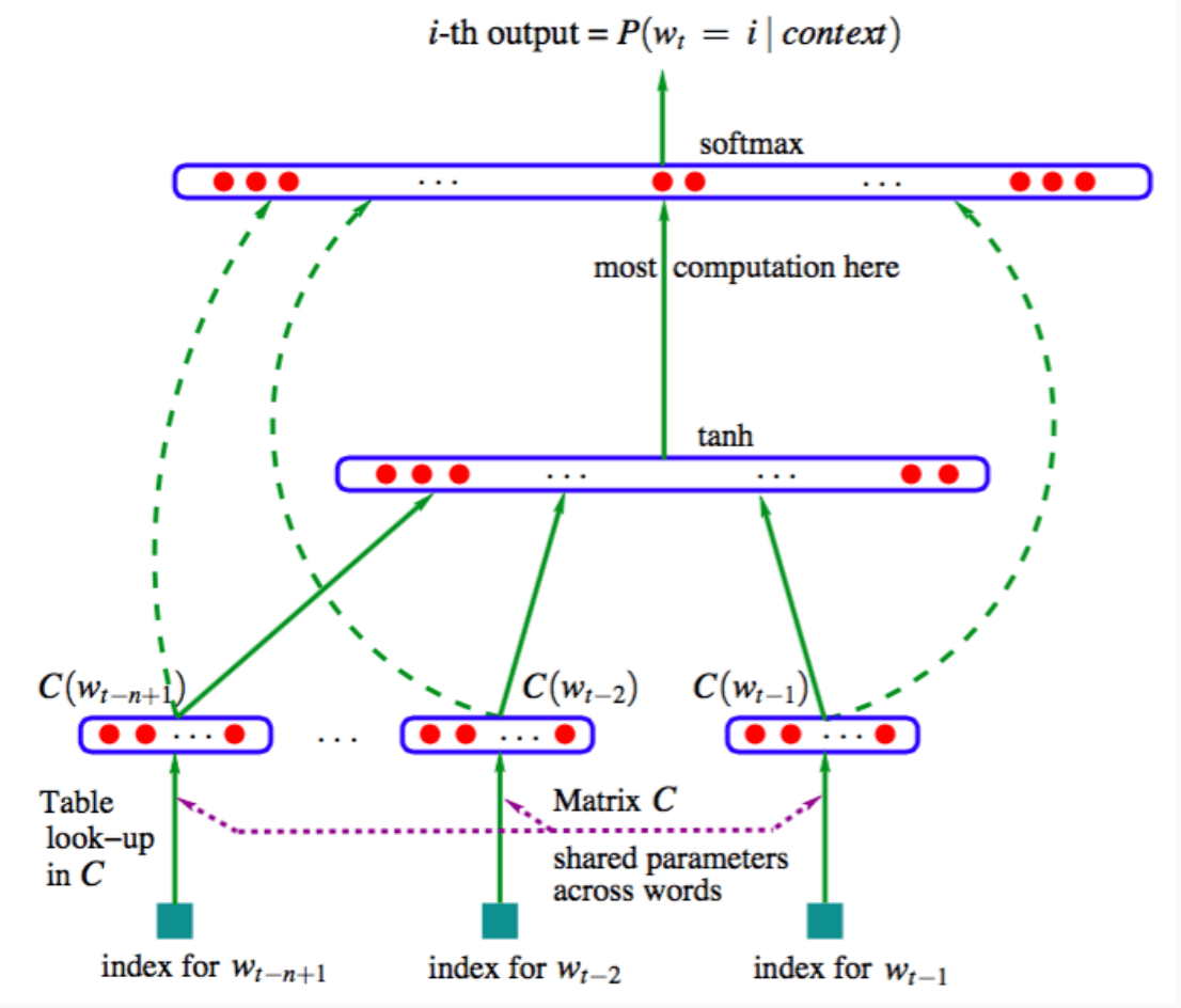
- \(C\) 为词嵌入.
- 参数量: 词汇量 \(V\approx18000\), 嵌入维数 \(d\) 为 \(30\) 或 \(60\), 隐层维数 \(H\) 为 \(50\) 或 \(100\), 上下文长度 \(n=6\), 故总参数量在 4M ~ 8M.
It is still an N-gram LM, but why it works better?
- 多层的结构使得特征可以组合
- we can search through a lot more conjunctive features through high dimensional feature representations, especially for neural models the amazing word embeddings!
- 可以同时训练词嵌入和 FFNN
实际上, 该网络并没有为序列建模, 因为 \(h_{1:n-1}\) 中的词汇只是简单地求和, 并未考虑顺序.
3.3 Convolutional networks
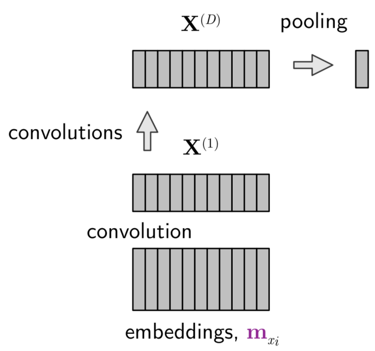
设输入词嵌入 (列向量) 序列 \(X^{(0)}=(m_1,m_2,\dots,m_{t-1})\in\R^{d\times(t-1)}\), 我们用一个滑动窗口扫过整个句子: \[ X^{(\ell)}[k,m] := f\pqty{ b_k + \sum_{i=1}^{\textsf{$d$ or $K$}} \sum_{j=1}^{{\sf sw}} C_{k}[i,j]\cdot X^{(\ell-1)}[i,m+j-1] } \in \R^{K\times(t-1)} . \] 每组 \((b_k\in\R,C_k\in\R^{(\textsf{\)d$ or \(K\)})})$ 都代表一个 filter (\(k=1,\dots,K\)); \({\sf sw}\) 是滑动窗口的宽.
我们一共进行 \(D\) 次卷积, 得到隐层 \(X^{(1)},\dots,X^{(D)}\). 最后用一个 max pool 或 average pool 得到一个向量: \[ z_i := \max_j X^{(D)}[i,j],\quad\textsf{or}\quad z_i := \frac1{t-1} \sum_{j=1}^{t-1} X^{(D)}[i,j]. \] 最后用 softmax 得到概率.
3.4 Recurrent networks
能否更好地建模历史序列?
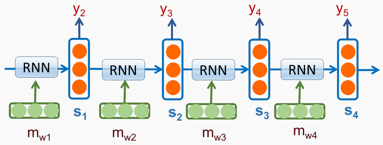
在每个词 \(m_i\) 处, 用一个隐状态 \(s_{i-1}\) 来编码历史序列 \(h_{1:i-1}\), 并迭代地更新:
- \(s_0=0\).
- \(s_i=\delta(m_iW_m + s_{i-1}W_s +
b)\).
- 输出 \(p(w_{i+1}\mid h_{1:i})=\operatorname{softmax}(s_iW_p)\).
该 RNN 结构如下:
朴素 RNN 的缺点是:
- Gradients decrease rapidly as they get pushed back. (梯度消失)
- Hidden states tend to change a lot on each iteration. (快速遗忘)
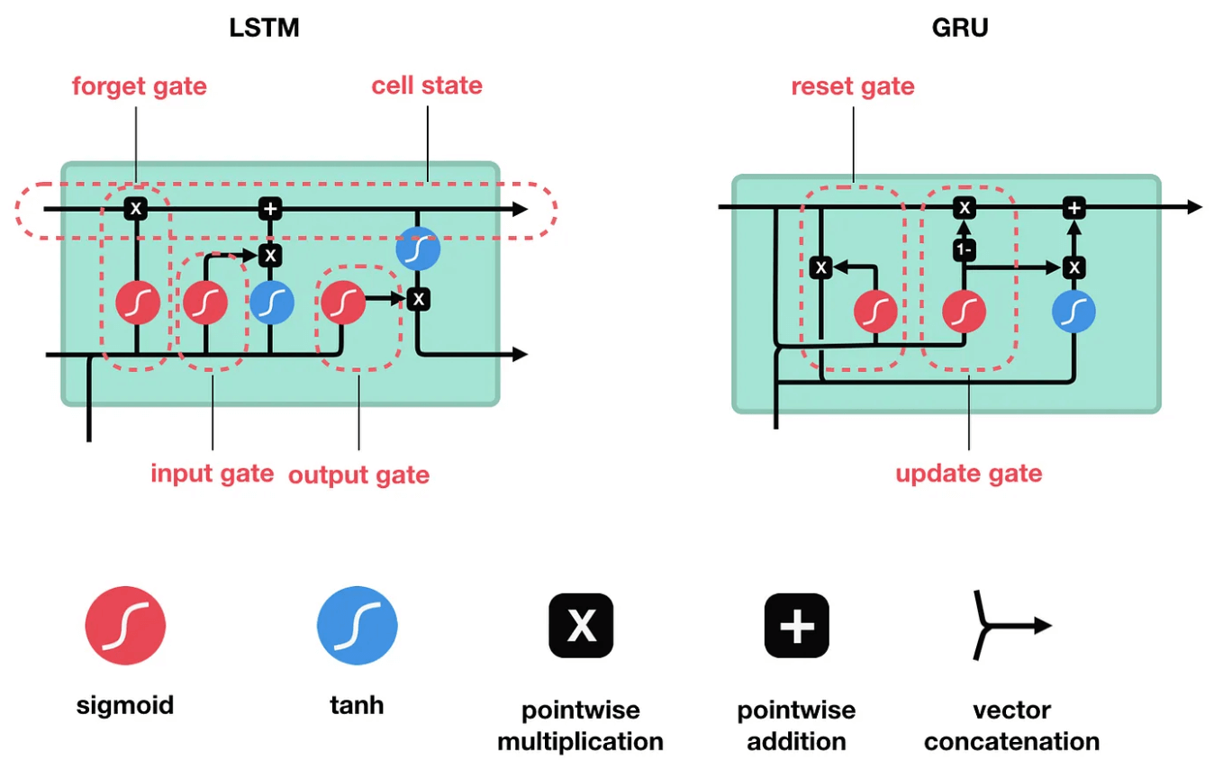
Long Short-Term Memory (LSTM, Hochreiter and Schmidhuber 1997)
引入了一些 gates 和加法连接来保持长期记忆. GRUs (Cho et al., 2014)
简化了 LSTM 的结构. 它们如下图所示
stronger modeling regarding history \(\Rightarrow\) from fixed \(t\) to almost all history
3.5 Contextual representations
Words may have multiple distinct meanings, 因此只用一个向量编码一个单词是不够的.
Go deeper!
 |
 |
|---|
Michael Phi, Illustrated Guide to LSTM’s and GRU’s: A step by step explanation (@medium, 2018).↩︎