流体模拟
如无特殊说明, 本文图片均取自课程 PPT.
6 流体模拟
6.1 两种视角
流体的难点在于, 其在空间中连续分布, 因此需要选择合适的空间离散化方法. 流体的空间离散化有两种视角: Lagrange 和 Euler.
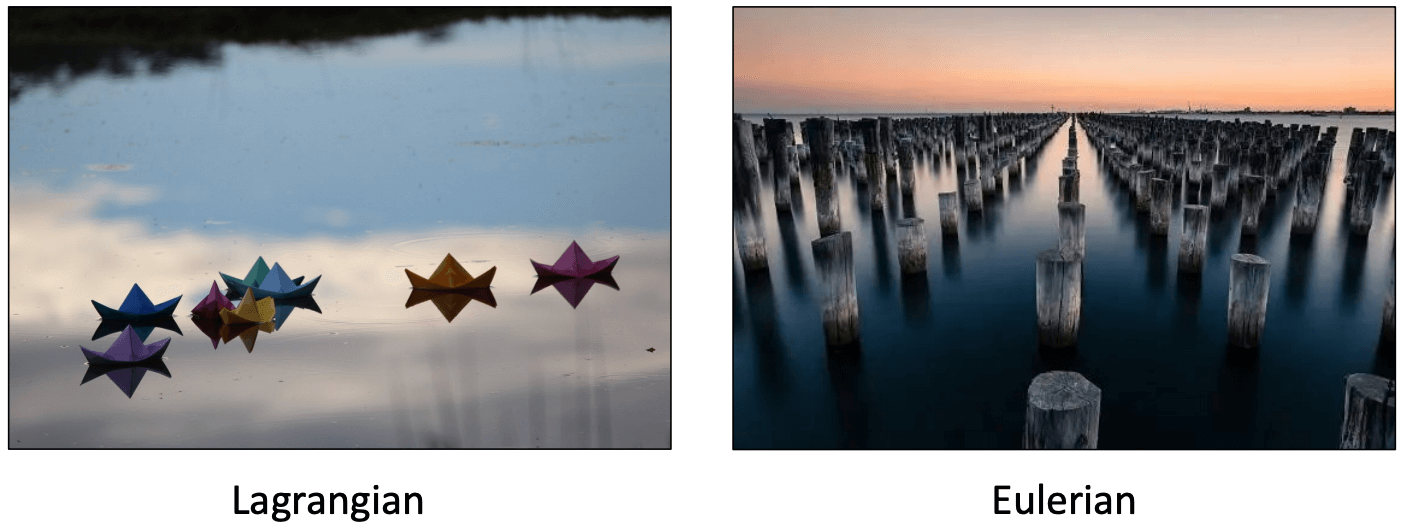
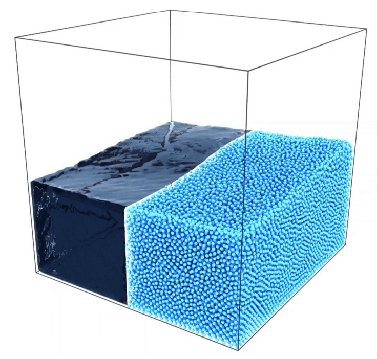
- Lagrange: 在流体上采样若干粒子 (类似于流体中的小船), 用粒子的运动代表流体的运动.
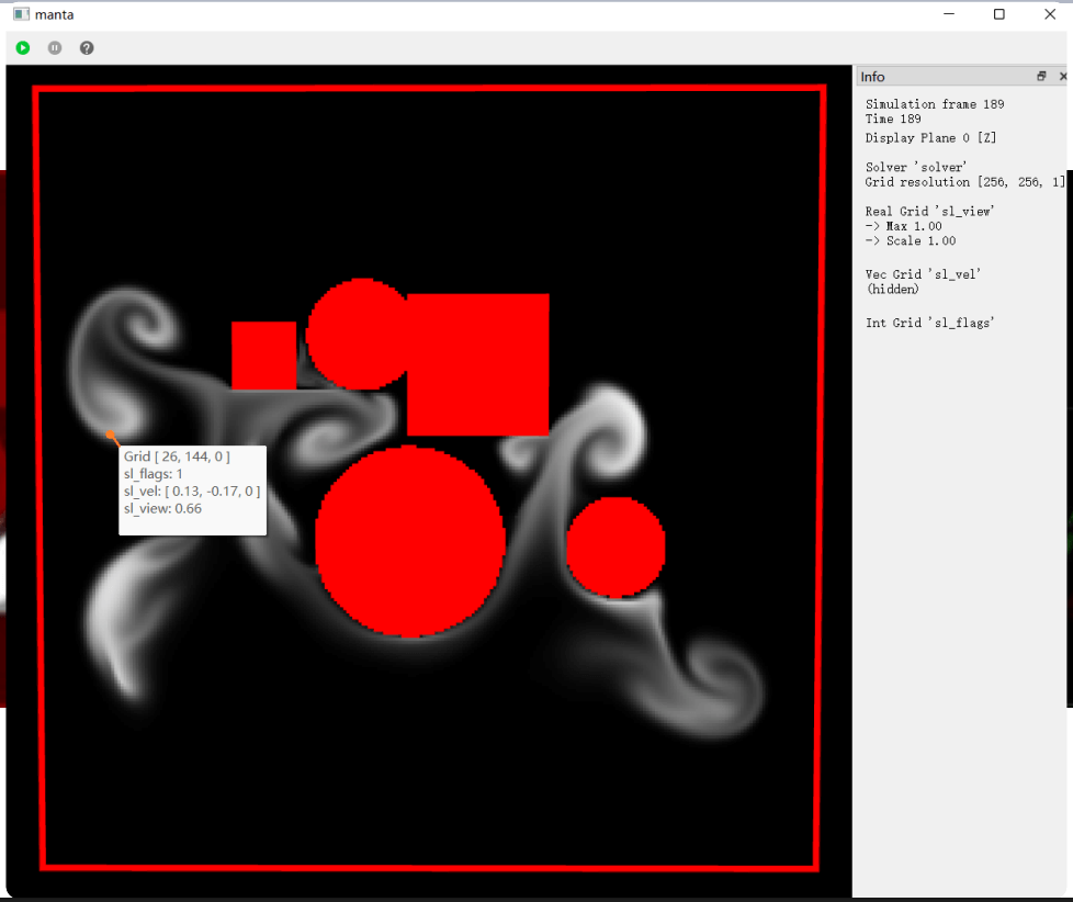
- Euler: 将空间离散化为网格 (类似与固定的木桩), 记录格点处流体的速度以代表流体的运动.
两者孕育了不同的仿真方法, 适合不同的场景 (下左为 Lagrange 的粒子流体模拟; 右为 Euler 的烟雾模拟).
 |
 |
|---|
6.2 运动方程
设流体的密度场为 \(\rho(x,t)\), 速度场为 \(v(x,t)\), 则流体的运动由 Navier-Stokes 方程描述: \[ \rho \frac{Dv}{Dt} = \underbrace{-\nabla p}_{\sf pressure} {} + {} \underbrace{\rho g}_{\sf gravity} {}+{} \underbrace{\mu\Delta v}_{\sf viscosity}. \] 其本质是 Newton 第二定律. 其中,
左侧的 \(D/Dt\) 是速度的 material derivative, 指的是流体的一个粒子处 (该粒子可能在运动) 的物理量随时间的变化, 属于 Lagrange 视角. 而偏导数 \(\partial/\partial t\) 指的在某个固定点上, 某个物理量随时间的变化, 属于 Euler 视角. 两者有关联: \[ \Align{ \frac{Dq}{Dt} &= \pdv{q}{t} + \pdv{q}{x}\pdv{x}{t} \\ &= \pdv{q}{t} + \underbrace{(v\cdot\nabla)q}_{\textsf{advective term}}. } \]
粘滞阻力 \(\mu\Delta v\) 关于 \(v\) 是线性的. 这是当流体粘性较低时的合理近似. 对于很粘的流体 (比如蜂蜜), 粘滞阻力是非线性的.
光 N-S 方程还不足以完全描述流体. 我们还需要一个质量守恒方程: \[ \pdv{\rho}{t} = -\nabla\cdot (\rho v). \] 上式右边展开为 \(-\rho\nabla\cdot v-(v\cdot\nabla)\rho\). 其中速度的散度 \(\nabla\cdot v\) 对于不可压缩 (imcompressible) 流体来说等于零. 借助质量守恒方程, 不可压缩的几种等价说法是 \[ \nabla\cdot v = 0,\quad\textsf{或者}\quad \pdv{\rho}{t} = -(v\cdot\nabla)\rho,\quad\textsf{或者}\quad \frac{D\rho}{Dt} = 0. \]
- 大部分流体, 甚至某些气体都几乎是不可压缩的, 为了方便模拟, 我们认为它们就是不可压缩的. 但对于高速流体就要考虑它的压缩了.
总之, 我们得到了两个方程 \[ \left\{\Align{ \rho \frac{Dv}{Dt} &= -\nabla p + \rho g + \mu\Delta v, \\ \nabla\cdot v &= 0. }\right. \] 下面列出了偏微分方程的三种边界条件:
- (Dirichlet) 边界处的值给定 \(f_{\partial\Omega}(x,t)=C(x,t)\).
- (Neumann) 边界处的方向导数给定 \(\displaystyle\pdv{f_{\partial\Omega}}{n}(x,t)=\lr{n,\nabla f_{\partial\Omega}(x,t)}=C(x,t)\).
- (Robin) 结合两者 \(af_{\partial\Omega}(x,t)+b\displaystyle\pdv{f_{\partial\Omega}}{n}(x,t)=C(x,t)\).
7 Euler 网格法
7.1 网格表示与有限差分
Euler 视角将物理量 (密度、压强、温度、速度等) 存储在一个网格里. 这里以二维为例, 网格边长为 \(d\), 物理量 \(f\) 在 \((i,j)\) 单元处的值记作 \(f_{i,j}\) (这里以二维情形为例, 三维的是类似的).
物理量的偏导数可以用 central differencing 公式得到: \[ \pdv{f_{i,j}}{x} = \frac{f_{i+1,j}-f_{i-1,j}}{2d} \mod{\mathcal{O}(d^2)}. \] Laplace 算子为 \[ \Delta f_{i,j} = \frac{f_{i+1,j}+f_{i-1,j}+f_{i,j+1}+f_{i,j-1}-4f_{i,j}}{d^2}. \] 网格上的 Dirichlet 边界条件是很简单的, 只需把网格边界处的物理量值固定下来 (作为已知) 即可; Neumann 条件则是额外给出了一些 (关于边界附近物理量的) 方程.
求解 \(\Delta f=0\) 等价于在网格上求解线性系统: \[ L f = b, \] 其中 \(f\) 是未知物理量组成的矩阵, \(L\) 是代表 Laplace 算子的已知矩阵, \(b\) 是边界条件给出的已知物理量.
求解扩散方程 \(\partial f/\partial t=a\Delta f\) 可以用迭代法: \[ (I+ah L) f^{(k+1)} = f^{(k)} + ahb. \] Staggered grid 将速度存储在网格的边上, 可以达到更高精度. 其中, 标量密度、压强仍存储在网格中心; 水平速度 \(U\) 存储在网格的竖边上; 竖直速度 \(V\) 存储在网格的横边上, 如下图.
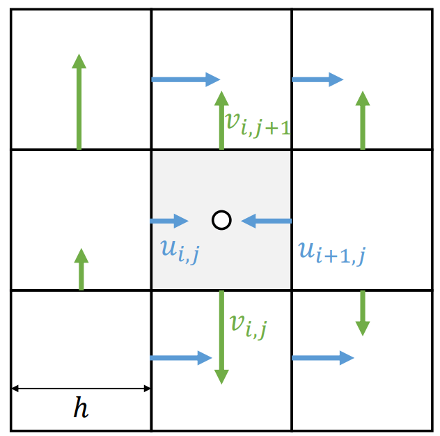
任意一点的物理量通过双线性插值得到.
- 后文中, 小写 \(v\) 代表速度向量; 大写 \(U,V\) 代表速度的横竖分量, 有下标的 \(U_{i,j},V_{i,j}\) 代表 staggered grid 上的速度分量. (课程 PPT 中用小写的 \(u,v\) 代表速度分量.)
7.2 不可压缩粘性流的模拟
Euler 视角下的运动方程化为 \[ \left\{\Align{ \rho\pdv{v}{t} &= -\rho(v\cdot\nabla)v -\nabla p + \rho g + \mu\Delta v, \\ \nabla\cdot v &= 0. }\right. \] 将这个大的 PDF 分成几步求解:
- Update \(v\) by solving \(\partial v/\partial t=(v\cdot\nabla)v\) (advection)
- Update \(v\) by solving \(\partial v/\partial t=g\) (external acceleration)
- Update \(v\) by solving \(\partial v/\partial t=\mu/\rho\cdot\Delta v\) (viscosity or diffusion)
- Update \(v\) by solving \(\partial v/\partial t=-1/\rho\cdot\nabla p\), such that \(\nabla\cdot v=0\) (pressure projection)
7.2.1 Advection
Update \(v\) by solving \(\partial v/\partial t=(v\cdot\nabla)v\).
不幸的是, 用 Euler 视角求解该式是 unconditionally unstable 的. 我们需要采用 semi-Lagrange 视角. 注意到对流项是由于其他地方的粒子带着物理量运动到此处产生的. 我们追溯粒子上一步的位置以取得速度: \[ \Align{ x_0 &\leftarrow (i-0.5,j), \\ x_1 &\leftarrow x_0 - hU(x_0), \\ U_{i,j} &\leftarrow U(x_1), } \] (其中 \(u(x_1)\) 是双线性插值得到的) 示意图为如下左侧. 对于 \(V_{i,j}\) 同理.
 |
 |
|---|
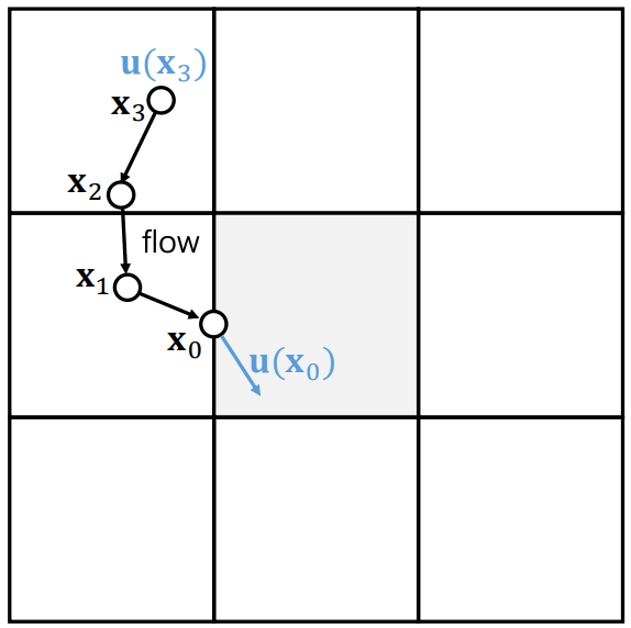
我们也可以对时间步 \(h\) 进行细分来达到更高精度, 如上图右侧, \[ \Align{ x_0 &\leftarrow (i-0.5,j), \\ x_1 &\leftarrow x_0 - \tfrac{h}{3} U(x_0), \\ x_2 &\leftarrow x_1 - \tfrac{h}{3} U(x_1), \\ x_3 &\leftarrow x_2 - \tfrac{h}{3} U(x_2), \\ U_{i,j} &\leftarrow U(x_3). } \] Semi-Lagrange 法在计算时可能遇到追溯到的点 \(x^{\sf old}\) 不在流体中的情形. 这可能由两方面原因导致:
- 流体从外部流入.
- 数值误差.
解决办法:
- 使用已知的边界条件.
- 从流体中最近的点外推 (extrapolate).
- Can do this extrapolation before advection at all grid points in the domain that aren't fluid.
- If fluid can move to a grid point that didn’t used to be fluid, make sure to do semi-Lagrange advection there using the extrapolated velocity
Semi-Lagrange 法会引入一种系统误差, 称为数值粘性 (numerical
viscosity). 考虑一维的对流方程 \[
\pdv{q}{t} - v\pdv{q}{x} = 0.
\] Euler 法的格子边长为 \(d\),
格点处的位置记作 \(x_i\), 物理量记作
\(q_i\). 不妨设 \(h<d/|v|\)
\[ \Align{ q_i^{\sf new} &= \frac{hv}{d} q_{i-1} + \pqty{1-\frac{hv}{d}} q_i, \\ \textsf{即 } q_i^{\sf new} &= q_i - hv \frac{q_i - q_{i-1}}{d}, } \] 将 \(q_i\) 在 \(x_i\) 处 Taylor 展开, \(q_{i-1}=q_i-d\pdv{q}{x}+\frac{d}{2}\pdv[2]{q}{x}+\mathcal{O}(d^3)\), 代入上式得到 \[ q_i^{\sf new} = q_i -hv \pdv{q}{x} + h\frac{vd}{2} \pdv[2]{q}{x} + \mathcal{O}(d^2), \] 复原到对流方程的形式, 我们有 \[ \underbrace{\frac{q_i^{\sf new} - q_i}{h}}_{\approx\partial q/\partial t} + v\pdv{q}{x} = \frac{vd}{2} \orange{\pdv[2]{q}{x}}, \] 方程右边的项非零, 即数值粘性. 关于数值粘性, Fluid Simulation (SIGGRAPH 2006 Course Notes) 这样说道:
So how bad is it? It depends on what we’re trying to simulate. If we’re trying to simulate a viscous fluid, which has plenty of natural dissipation already, then the extra numerical dissipation will hardly be noticed—and more importantly, looks plausibly like real dissipation. But, most often we’re trying to simulate nearly inviscid fluids, and this is a serious annoyance which keeeps smoothing the interesting features like small vortices from our flow. As bad as this is for velocity, in chapter 6 we’ll see it can be much much worse for other fluid variables.
7.2.2 External acceleration
Update \(v\) by solving \(\partial v/\partial t=g\).
直接把重力加速度累加到速度上: \[ V_{i,j} \leftarrow V_{i,j} + hg. \]
7.2.3 Viscosity or diffusion
Update \(v\) by solving \(\partial v/\partial t=\mu/\rho\cdot\Delta v\).
可以直接把 Laplacian 加到速度上: \[ U_{i,j} \leftarrow U_{i,j} + h\frac{\mu}{\rho} \frac{U_{i-1,j}+U_{i+1,j}+U_{i,j-1}+U_{i,j+1} - 4U_{i,j}}{d^2}. \] (对 \(V_{i,j}\) 同理) 如果 \(h\mu/\rho\) 比较大的话, 上式可能不稳定. 此时可以把时间步 \(h\) 细分, 比如 \[ \Align{ U_{i,j}^{\sf temp} &\leftarrow U_{i,j} + \frac{h}{2}\frac{\mu}{\rho} \frac{U_{i-1,j}+U_{i+1,j}+U_{i,j-1}+U_{i,j+1} - 4U_{i,j}}{d^2}, \\ U_{i,j}^{\sf new} &\leftarrow U_{i,j} + \frac{h}{2}\frac{\mu}{\rho} \frac{U_{i-1,j}^{\sf temp}+ U_{i+1,j}^{\sf temp}+ U_{i,j-1}^{\sf temp}+ U_{i,j+1}^{\sf temp}- 4U_{i,j}^{\sf temp} }{d^2}. \\ } \]
7.2.4 Pressure projection
Update \(v\) by solving \(\partial v/\partial t=-1/\rho\cdot\nabla p\), such that \(\nabla\cdot v=0\).
换言之, 求出 \(v^{\sf new}\) 满足 \(v^{\sf new}-v=-h/\rho\cdot\nabla p\) 且 \(\nabla\cdot v^{\sf new}=0\). 也即 \[ \nabla\cdot\pqty{v - \frac{h}{\rho}\nabla p} = 0, \] 或 Poisson 方程 \[ \Delta p = \frac{\rho}{h} \nabla v. \] 将其离散化, \[ 4p_{i,j} - p_{i-1,j} - p_{i+1,j} - p_{i,j-1} - p_{i,j+1} = \frac{\rho d}{h}(U_{i,j} - U_{i-1,j} + V_{i,j} - V_{i,j-1}), \] 等式右边是已知的, 由此得到关于 \(p\) 的线性方程组, 形如 \(Lx=b\). 其中:
- 向量 \(x\) 包含了所有流体点的压力
\(p_{i,j}\), 向量 \(b\) 包含了速度分量 \(U_{i,j},V_{i,j}\) 的线性组合.
需要注意如下边界条件:
- 邻居为空气. 表面处的压力为常值, 由于我们只关心压力梯度, 不妨设该常值为零. 故得到 Dirichlet 边界条件, 边界点 \(p_{i,j}=0\)[^tension-bd]. 在向量 \(x\) 中删去边界点的压力.
- 邻居为固体. 比如 \((i-1,j)\)
为固体. 对于无粘性流, 法向相对速度 \(U_{i,j}-U_{\sf solid}=0\) (no-stick).
对于粘性流, 相对速度 \((U_{i,j},V_{i,j})-(U_{\sf solid},V_{\sf
solid})=0\) (no-slip). 这是一个 Neumann 边界条件. 在实现上,
- Drop \(p_{i-1,j}\) and reduce coefficient of \(p_{i,j}\) by \(1\) (\(4\) to \(3\)),
- "No−stick": Only replace \(U_{i,j}\) (the right-hand side) with \(U_{\sf solid}\),
- "No−slip": Also replace \(V_{i,j}\) (the right-hand side) with \(V_{\sf solid}\).
- Laplace 矩阵 \(L\) 是半正定的稀疏矩阵, 可以使用预条件共轭梯度法 (PCG, preconditioned conjugate gradient), 预条件为 incomplete Cholesky preconditioner. [^tension-bd]: 若考虑表面张力, 则表面处的压力与表面的平均曲率有关.
最终, 解出 \(p\) 后更新 \(v\): \[ \Align{ U_{i,j} &\leftarrow U_{ij} - \frac{h}{\rho d}(p_{i,j} - p_{i-1,j}), \\ V_{i,j} &\leftarrow V_{ij} - \frac{h}{\rho d}(p_{i,j} - p_{i,j-1}). } \]
7.3 颜料与烟雾
水中的颜料 / 空中的烟雾, 额外受水的浮力. 此外要考虑浓度的对流: \[ \pdv{c}{t} = -(v\cdot\nabla)c. \] 浮力与温度有关, 经验公式为 \[ f_b = -\alpha c + \beta(T-T_{\sf amb}), \]
7.4 水
水的特点是它有一个明显的界面 / 自由表面 (free surface).
7.4.1 标记点
- Simplest approach is to use marker particles.
- Sample fluid volume with particles \(\{x_p\}\)
- At each time step, mark grid cells containing any marker particles as Fluid, rest as Empty or Solid.
- Move particles in incompressible grid velocity field (interpolating
as needed):
- \({\dd{x_p}}/{\dd{t}}=v(x_p)\), we can use Euler update (with Runge-Kutta 2)
7.4.2 水平集
在模拟的过程中维护一个 SDF 的水平集, 作为水的表面.
- Initialization \(\phi(x)\) (for e.g., Fast Sweeping Method [Zhao H 2005, A fast sweeping method for eikonal equations]).
- Advection: \(\partial\phi/\partial t=(u\cdot\nabla)c\).
- Reinitialization \(\|\nabla\phi(x)\|=1\).
然而水平集对数粘性性十分敏感. Level set advection is very sensitive to numerical diffusion. Over time, sharp features are smoothed away and even disappear: small holes can fill in, thin structures can vanish.
对流方程数值求解收敛性的一个必要条件是 CFL 条件 (Courant–Friedrichs–Lewy), 即 \(h\leq Cd/|v|\). 其中 \(C\) 是常数, 显式方法中一般取 \(C=1\).↩︎